Power Measurement and Energy Consumption Cost

POWER MEASUREMENT


Power is symbolize as (P). It is defined as the amount of energy consumed per unit time. The unit of power is known as theWatt (W). The average power that is absorbed by the load is measured by a wattmeter. Loads consume electric power, converting it to other forms such as mechanical work, heat, light, etc. Examples of loads are electrical appliances, such as light bulbs, electric motors, and electric heaters. When we are using AC, power is determined not only by the r.m.s. values of the voltage and current, but also by the phase angle which will determine the power factor.

As I said, wattmeter is the device used to measure electrical power. This consists of current coil and the voltage coil. A current coil with very low impedance is connected in series with the load. This low impedance or ideally zero results to a very high current and zero voltage. The voltage coil has a very high impedance is connected in parallel. This high impedance or ideally infinite has a high voltage and a zero current. In a wattmeter, the current coil helps in measuring current and the potential coil is used for measuring voltage. A wattmeter does a complex job. Aside for measuring the power flowing through an electrical circuit, it also simultaneously measures the voltage and current values and multiplies them to give power in watts.


ELECTRICITY CONSUMPTION COST


Every appliance we have in our house has its own corresponding power. This power really matters on how much we pay in our electric bills that is why it is important to know how much power present in our appliance. Since we are paying for the electric energy over a period of time, we have to consider how long we use our appliances in our house.

Typical wattages if various appliances:

Aquarium = 50–1210 Watts
· Clothes washer = 350–500
· Clothes dryer = 1800–5000
· Fans Ceiling = 65–175
· Window = 55–250
· Furnace = 750
· Whole house = 240–750

· Hair dryer = 1200–1875
· Heater (portable) = 750–1500
· Clothes iron = 1000–1800
· Microwave oven = 750–1100
· Personal computer
· CPU - awake / asleep = 120 / 30 or less
· Monitor - awake / asleep = 150 / 30 or less
· Laptop = 50
· Radio (stereo) = 70–400
· Refrigerator (frost-free, 16 cubic feet) = 725
· Televisions (color)
· 19" = 65–110
· 27" = 113
· 36" = 133
· 53" - 61" Projection = 170
· Flat screen = 120
· Toaster = 800–1400
· VCR/DVD = 17–21 / 20–25
· Vacuum cleaner = 1000–1440




How is energy use of Home Appliances calculated?

TIPS TO CONSERVE ENERGY AND TO SAVE MONEY!!


Unplug electronic appliances and gadgets when not in use.

When buying new appliances, be sure to purchase energy-efficient


Lessen the hours of using the appliances.


Leave thermostat’s fan switch on “auto”.


Replace light bulbs with CFL’s.


Set the thermostats of the refrigerator at the appropriate temperature.


Clean or replace furnace and air-conditioner filters regularly, following
manufacturer's instructions.


Have self-discipline.

LEARNINGS:
I've learned that the more wattage, the more power, or equivalently the more electrical energy is used per unit time. High energy consumption will result to high electricity bill. I realized that we also need to conserve energy to decrease the quantity of energy used and also, we must use appliances in our house efficiently. Appliances that generate heat contributes high power such as flat iron, rice cooker, and etc.

Three-Phase Circuits

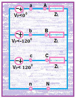
From our past lessons, we always dealt with single-phase circuits. A single-phase ac power system is consists of a generator connected to a pair of wires to a load. These pair of wires is what we called transmission line. Polyphase are circuits or systems which the ac sources operate at the same frequency but different phases. A two-phase system is produced by a generator consisting of two coils placed perpendicular to each other so that thee voltage generated by one lags the other by 900 while a three-phase system is produced by a generator consisting of three sources having the same amplitude and frequency but out of phase with each other by 1200.
See the difference of the said three systems above by means of figures:

Single-phase two wire system

Two-phase three wire system

Three-phase four wire system

In our household, we single-phase three wire system because the terminal voltages have the same magnitude and the same phase. Also, whether it is single-phase, two-phase or three-phase system, we can’t put load as many as we can. We must also consider the power supplied by the source if it is enough to accommodate certain number of loads. Example of this is a power amplifier we’ve made; we have 70V and 8A a total of 560W power. Our power amplifier is 100W so; I can say that there must only 10 100-W power amplifier that must be put in the circuit

BALANCED THREE-PHASE VOLTAGES


Three-phase voltage is often produced by a three-phase ac generator. Balanced phase voltages are equal in magnitude but different in phase angle because they are out of phase with each other by 1200. A three-phase system is equivalent o three single-phase circuits. A voltage sources can be connected either wye-connected or delta-connected

DELTA CONNECTION

WYE CONNECTION

There are also two types of phase sequence, one is positive or abc sequence in which Van leads Vbn which in turn leads Vcn. The other one is negative or acb sequence in which Van leads Vcn which in turn leads Vbn. This phase sequence is the time order in which the voltages pass through their respective maximum values.

POSITIVE SEQUENCE

NEGATIVE SEQUENCE

NOTE:


A balanced load is one in which the phase impedances are equal in magnitude and in phase. Wye connected load has impedances connected in neutral node while delta connected has impedances connected around a loop.


DEFINITION OF IMPORTANT TERMS:


Line current - current flowing from the generator to the load in each
transmission line
line voltage - the voltage between in each pair of lines
phase current – current flowing through each phase
phase voltage – voltage of each phase


BALANCED WYE-WYE CONNECTION


A balanced Wye-Wye system is a three-phase system with a balanced connected source and a balance connected load. We can solve for its line current by getting a single-phase loop from the circuit and applying KVL.

Summary: 

BALANCED DELTA-DELTA CONNECTION


A balanced delta-delta system is one in which both the balanced source and balanced load are delta-connected. For easy analyzing the delta-delta connected circuit, transform both the source and the load to their wye equivalent.

Summary: 

BALANCED DELTA-WYE CONNECTION


A balanced delta-wye system consists of a balanced delta-connected source and a balanced wye-connected load. There are also the line voltages as well as the phase voltages. We can generate an equation through getting a loop from the circuit and this may help us solved for the line currents. Like in other connections, we may also transform delta-connected source to wye-connected source.

Summary: 

LEARNINGS:


After the partial discussion of three-phase system, I’ve learned that in a wye-connected balanced source, line currents and phase currents are equal while in a delta-connected balanced source, line voltage and phase voltage is equal. For solving, its easy to solve the required parameters if the system is a wye-wye connection because it has a single-phase equivalent circuit that is easy to analyze. Also, I’ve found out that the electric power is generated and distributed in three-phase at the standard operating frequency.

Power Factor Correction

When the need arises to correct for poor power factor in an AC power system, you probably won’t have the luxury of knowing the load’s exact inductance in henrys to use for your calculations. You may be fortunate enough to have an instrument called a power factor meter to tell you what the power factor is (a number between 0 and 1), and the apparent power (which can be figured by taking a voltmeter reading in volts and multiplying by an ammeter reading in amps). In less favorable circumstances you may have to use an oscilloscope to compare voltage and current waveforms, measuring phase shift in degrees and calculating power factor by the cosine of that phase shift.

Most likely, you will have access to a wattmeter for measuring true power, whose reading you can compare against a calculation of apparent power (from multiplying total voltage and total current measurements). From the values of true and apparent power, you can determine reactive power and power factor. Let’s do an example problem to see how this works:

Wattmeter reads true power; product of voltmeter and ammeter readings yields appearant power.

First, we need to calculate the apparent power in kVA. We can do this by multiplying load voltage by load current:

As we can see, 2.308 kVA is a much larger figure than 1.5 kW, which tells us that the power factor in this circuit is rather poor (substantially less than 1). Now, we figure the power factor of this load by dividing the true power by the apparent power:

Using this value for power factor, we can draw a power triangle, and from that determine the reactive power of this load:

Reactive power may be calculated from true power and appearant power.

To determine the unknown (reactive power) triangle quantity, we use the Pythagorean Theorem “backwards,” given the length of the hypotenuse (apparent power) and the length of the adjacent side (true power):

If this load is an electric motor, or most any other industrial AC load, it will have a lagging (inductive) power factor, which means that we’ll have to correct for it with a capacitor of appropriate size, wired in parallel. Now that we know the amount of reactive power (1.754 kVAR), we can calculate the size of capacitor needed to counteract its effects:

Rounding this answer off to 80 µF, we can place that size of capacitor in the circuit and calculate the results

Parallel capacitor corrects lagging (inductive) load.

An 80 µF capacitor will have a capacitive reactance of 33.157 Ω, giving a current of 7.238 amps, and a corresponding reactive power of 1.737 kVAR (for the capacitor only). Since the capacitor’s current is 180oout of phase from the the load’s inductive contribution to current draw, the capacitor’s reactive power will directly subtract from the load’s reactive power, resulting in:

This correction, of course, will not change the amount of true power consumed by the load, but it will result in a substantial reduction of apparent power, and of the total current drawn from the 240 Volt source:

Power triangle before and after capacitor correction.

The new apparent power can be found from the true and new reactive power values, using the standard form of the Pythagorean Theorem:

This gives a corrected power factor of (1.5kW / 1.5009 kVA), or 0.99994, and a new total current of (1.50009 kVA / 240 Volts), or 6.25 amps, a substantial improvement over the uncorrected value of 9.615 amps! This lower total current will translate to less heat losses in the circuit wiring, meaning greater system efficiency (less power wasted).

True, Reactive, and Apparent Power

We know that reactive loads such as inductors and capacitors dissipate zero power, yet the fact that they drop voltage and draw current gives the deceptive impression that they actually do dissipate power. This “phantom power” is called reactive power, and it is measured in a unit called Volt-Amps-Reactive (VAR), rather than watts. The mathematical symbol for reactive power is (unfortunately) the capital letter Q. The actual amount of power being used, or dissipated, in a circuit is called true power, and it is measured in watts (symbolized by the capital letter P, as always). The combination of reactive power and true power is called apparent power, and it is the product of a circuit’s voltage and current, without reference to phase angle. Apparent power is measured in the unit of Volt-Amps (VA) and is symbolized by the capital letter S.

As a rule, true power is a function of a circuit’s dissipative elements, usually resistances (R). Reactive power is a function of a circuit’s reactance (X). Apparent power is a function of a circuit’s total impedance (Z). Since we’re dealing with scalar quantities for power calculation, any complex starting quantities such as voltage, current, and impedance must be represented by their polar magnitudes, not by real or imaginary rectangular components. For instance, if I’m calculating true power from current and resistance, I must use the polar magnitude for current, and not merely the “real” or “imaginary” portion of the current. If I’m calculating apparent power from voltage and impedance, both of these formerly complex quantities must be reduced to their polar magnitudes for the scalar arithmetic.

There are several power equations relating the three types of power to resistance, reactance, and impedance (all using scalar quantities):

Please note that there are two equations each for the calculation of true and reactive power. There are three equations available for the calculation of apparent power, P=IE being useful only for that purpose. Examine the following circuits and see how these three types of power interrelate for:

Resistive load only:

True power, reactive power, and apparent power for a purely resistive load.

Reactive load only:

True power, reactive power, and apparent power for a purely reactive load.

Resistive/reactive load:

True power, reactive power, and apparent power for a resistive/reactive load.

These three types of power—true, reactive, and apparent—relate to one another in trigonometric form. We call this the power triangle:

Power triangle relating appearant power to true power and reactive power.

Using the laws of trigonometry, we can solve for the length of any side (amount of any type of power), given the lengths of the other two sides, or the length of one side and an angle.

REVIEW:
Power dissipated by a load is referred to as true power. True power is symbolized by the letter P and is measured in the unit of Watts (W).

Power merely absorbed and returned in load due to its reactive properties is referred to as reactive power. Reactive power is symbolized by the letter Q and is measured in the unit of Volt-Amps-Reactive (VAR).

Total power in an AC circuit, both dissipated and absorbed/returned is referred to as apparent power. Apparent power is symbolized by the letter S and is measured in the unit of Volt-Amps (VA).

These three types of power are trigonometrically related to one another. In a right triangle, P = adjacent length, Q = opposite length, and S = hypotenuse length. The opposite angle is equal to the circuit’s impedance (Z) phase angle.

Maximum Power Transfer Theorem

The Maximum Power Transfer Theorem is not so much a means of analysis as it is an aid to system design. Simply stated, the maximum amount of power will be dissipated by a load resistance when that load resistance is equal to the Thevenin/Norton resistance of the network supplying the power. If the load resistance is lower or higher than the Thevenin/Norton resistance of the source network, its dissipated power will be less than maximum.

This is essentially what is aimed for in radio transmitter design , where the antenna or transmission line “impedance” is matched to final power amplifier “impedance” for maximum radio frequency power output. Impedance, the overall opposition to AC and DC current, is very similar to resistance, and must be equal between source and load for the greatest amount of power to be transferred to the load. A load impedance that is too high will result in low power output. A load impedance that is too low will not only result in low power output, but possibly overheating of the amplifier due to the power dissipated in its internal (Thevenin or Norton) impedance.

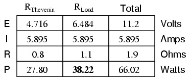
Taking our Thevenin equivalent example circuit, the Maximum Power Transfer Theorem tells us that the load resistance resulting in greatest power dissipation is equal in value to the Thevenin resistance (in this case, 0.8 Ω):

With this value of load resistance, the dissipated power will be 39.2 watts:

If we were to try a lower value for the load resistance (0.5 Ω instead of 0.8 Ω, for example), our power dissipated by the load resistance would decrease:

Power dissipation increased for both the Thevenin resistance and the total circuit, but it decreased for the load resistor. Likewise, if we increase the load resistance (1.1 Ω instead of 0.8 Ω, for example), power dissipation will also be less than it was at 0.8 Ω exactly:

If you were designing a circuit for maximum power dissipation at the load resistance, this theorem would be very useful. Having reduced a network down to a Thevenin voltage and resistance (or Norton current and resistance), you simply set the load resistance equal to that Thevenin or Norton equivalent (or vice versa) to ensure maximum power dissipation at the load. Practical applications of this might include radio transmitter final amplifier stage design (seeking to maximize power delivered to the antenna or transmission line), a grid tied inverterloading a solar array, or electric vehicle design (seeking to maximize power delivered to drive motor).
The Maximum Power Transfer Theorem is not: Maximum power transfer does not coincide with maximum efficiency. Application of The Maximum Power Transfer theorem to AC power distribution will not result in maximum or even high efficiency. The goal of high efficiency is more important for AC power distribution, which dictates a relatively low generator impedance compared to load impedance.
Similar to AC power distribution, high fidelity audio amplifiers are designed for a relatively low output impedance and a relatively high speaker load impedance. As a ratio, "output impdance" : "load impedance" is known as damping factor, typically in the range of 100 to 1000.


Maximum power transfer does not coincide with the goal of lowest noise. For example, the low-level radio frequency amplifier between the antenna and a radio receiver is often designed for lowest possible noise. This often requires a mismatch of the amplifier input impedance to the antenna as compared with that dictated by the maximum power transfer theorem.

Instantaneous Power

The second chapter of this semester has been opened! Now we have discussed about instantaneous power. We were first had our insights about what instantaneous power is. Unlike DC power, instantaneous power is only present in an AC powered circuit. Alternating power or AC power by definition is a power that is changing by a definite amount over a period of time. And in every point in time, there is a particular designated power as well.




We begin our exploration of sinusoidal power calculations with the genaric circuit in the following figure. In here, v and i are steady-state sinusoidal signals. By using the passive sign convention (PSC), the power at any instant of time is given by: 

                                                                               p=vi

This equation describes instantaneous power. Recall that if the reference direction of the current is in the direction of the voltage rise, must be written with a minus sign. Instantaneous power is always measured in watts when the voltage is measured in volts and the current is measured in amperes. Two expressions of phase angles of v and i are written as


v=Vmcos(ωt+θv),v=Vmcos⁡(ωt+θv), (1.2)


i=Imcos(ωt+θi),i=Imcos⁡(ωt+θi), (1.3)



In these two expressions, θvθv is the voltage phase angle, and θiθi is the current phase angle.


While working in the sinusoidal steady state, a convenient reference for zero time may be chosen. Engineers who design systems that transfer large amounts of power have found it convenient to use a zero time that corresponds to the instant the current is passing through a positive maximum. By choosing such a reference time, a shift of both voltage and current by θiθi is required. Now, Eqs. 1.2 and 1.3 become



v=Vmcos(ωt+θv−θi)v=Vmcos⁡(ωt+θv−θi) (1.4)

i=Imcos(ωt)i=Imcos⁡(ωt) (1.5)



If Eqs. 1.4 and 1.5 are substituted into Eq. 1.1, the expression for the instantaneous power now becomes

p=VmImcos(ωt+θv−θi)cos(ωt)p=VmImcos⁡(ωt+θv−θi)cos⁡(ωt) (1.6)


Eq. 1.6 can be used to solve for average power the way it is; however, by applying a few simple trigonometric identities the instantaneous power equation can be simplified. Using cosine's product identity gives

cos(α)cos(β)=12cos(α−β)+12cos(α+β)cos⁡(α)cos⁡(β)=12cos⁡(α−β)+12cos⁡(α+β)



Letting
α=ωt+θv−θiα=ωt+θv−θi and
β=ωtβ=ωt provides


p=VmIm2cos(θv−θi)+VmIm2cos(2ωt+θv−θi)p=VmIm2cos⁡(θv−θi)+VmIm2cos⁡(2ωt+θv−θi) (1.7)



Lastly, using the cosine angle-sum identity


cos(α+β)=cos(α)cos(β)−sin(α)sin(β)cos⁡(α+β)=cos⁡(α)cos⁡(β)−sin⁡(α)sin⁡(β)



to expand the second term on the right-hand side of Eq 1.7, which gives


p=VmIm2cos(θv−θi)+VmIm2cos(θv−θi)cos(2ωt)−VmIm2sin(θv−θi)sin(2ωt)p=VmIm2cos⁡(θv−θi)+VmIm2cos⁡(θv−θi)cos⁡(2ωt)−VmIm2sin⁡(θv−θi)sin⁡(2ωt) (1.8)

Relationship Between Current, Power, and Voltage

Figure 1.2 below depicts the relationship between i, v, and p, assuming that θv=60∘θv=60∘ and θi=0∘θi=0∘. The frequency of the instantaneous power is twice the frequency of the current or voltage. This depiction also follows from the second two terms on the right side of Eq. 1.8. This means that the instantaneous power goes through two complete cycles for every cycle of either the current or the voltage. If you look at Fig. 1.2, the instantaneous power can be negative for a portion of each cycle, even if the network between the terminals is passive. In a passive network, this negative power implies that the energy being stored in the inductors or capacitors is now being extracted. While the instantaneous power varies with time in the sinusoidal steady-state of a circuit, this causes some vibration in some motor-driven appliances. Due to this vibration in these appliances, resilient motor mountings are required to reduce any excessive vibration.

Average and Reactive Power

Eq. 1.8 can now be utilized to find the average power at the terminals of the circuit, as well as establish the concept of reactive power. Noting that the equation has three terms, it can be rewritten as

p=P+Pcos(2ωt)−Qsin(2ωt),p=P+Pcos⁡(2ωt)−Qsin⁡(2ωt), (1.9)


Where

Average (real) power
P=VmIm2cos(θv−θi)P=VmIm2cos⁡(θv−θi) (1.10)


Reactive power
Q=VmIm2sin(θv−θi)Q=VmIm2sin⁡(θv−θi) (1.11)



P is called the average power, and Q is called the reactive power. Average power is also known as real power, because it is the actual power in a circuit that is transformed from electric to nonelectric energy. The average power associated with sinusoidal signals is the average of the instantaneous power over one period, or


P=1T∫t0+Tt0pdt,P=1T∫t0t0+Tpdt, (1.12)




Where T is the period of the sinusoidal varying function. The bounds of the integral indicate that integration can be made at any convenient time
t0t0 and integration must be bounded exactly one period later. To grasp a better understanding of all the terms in Eq. 1.9 and the relationships they hold, we will need to examine the power in circuits that are purely resistive, purely inductive, and purely capacitive.


Purely Resistive Circuits

If a circuit between terminals is purely resistive, the current and voltage are in phase
(θv=θi)(θv=θi). Thus, Eq. 1.9 can be reduced to



p=P+Pcos(2ωt)p=P+Pcos⁡(2ωt) (1.13)



This is referred to as the instantaneous real power. Figure 1.3 is a graph of the instantaneous real power for a purely resistive circuit, assuming
ω=377rad/sω=377rad/s. The average power, P, is the average of p, over one period. This can be seen by looking at the graph where P=1 for the circuit. From the Fig 1.3, instantaneous real power can never be negative; in other words, power cannot be removed from a purely resistive network. While the power cannot be removed, it is however, dissipated in the form of thermal energy.

Purely Inductive Circuits

Now, if the circuit between the terminals is purely inductive, the current and voltage are out of phase by 90∘.90∘.The current of the circuit lags the voltage by 90∘90∘ (θi=θv−90∘).(θi=θv−90∘). The instantaneous power equation can be reduced to


p=−Qsin(2ωt)p=−Qsin⁡(2ωt) (1.14)



In this purely inductive circuit, the average power is zero. This means that no transformation of energy from electric to nonelectric energy takes place. The power at the terminals is continually exchanged between the circuit and the power source driving the circuit at a frequency of
2ω.2ω. What this means, is that when p is positive, energy is stored in the magnetic fields associated with the inductive elements, and when p is negative, energy is being removed from the magnetic fields.


Power associated with purely inductive circuits is known as the reactive power Q. Reactive power comes from the characterization of an inductor as a reactive element. To differentiate between average power and reactive power, units watt (W) for average power and var (volt-amp reactive, or VAR) for reactive power are used. Figure 1.4 depicts the instantaneous power for a purely inductive circuit, assuming ω=377rads/sω=377rads/sand Q = 1 VAR.

Purely Capacitive Circuits

In this purely capacitive circuit, the current and voltage are
90∘90∘ out of phase with each other. In this case, the current leads the voltage by exactly
90∘90∘ (θi=θv+90∘)(θi=θv+90∘). The expression of this instantaneous power is given by


p=−Qsin(2ωt)p=−Qsin⁡(2ωt) (1.15)



In this circuit, there is no transformation of energy from electric to nonelectric energy because the average power is zero. In a purely capacitive circuit, the power is continually transferred between the source delivering power and to the electric field associated with the capacitive elements. Figure 1.5 depicts the instantaneous power for a purely capacitive circuit, assuming ω=377rads/sω=377rads/s and Q = -1 VAR.

Understanding the Power Factor

This angle (θv−θi)(θv−θi) has a significant role in computing both the average and the reactive power and is known as the power factor angle. Taking the cosine of this angle gives what is known as the power factor, shortened to pf, and taking the sine of this angle is known as the reactive factor, shortened to rf. This can be denoted as:


pf=cos(θv−θi)pf=cos⁡(θv−θi) (1.16)


rf=sin(θv−θi)rf=sin⁡(θv−θi) (1.17)


To completely describe the power factor angle, either lagging power factor or leading power factor terms are used. If the power factor lags, the current lags voltage (i.e. an inductive load is present). On the other hand, if the power factor leads, the current leads voltage (i.e. a capacitive load is present).

Wew. That was a hell of a research! I think my power is drained too. Got to go to sleep then!

Thévenin's Theorem with dependent sources (AC Analysis)

Thévenin's Theorem is a lot work itself, how much more if we had to add dependent sources. The introduction of dependent sources complicates the calculation and process in solving for the thevenins impedance (Zth).

Having dependent source/s twitches the process of Thévenin's theorem. 

1. Determine Voc (Vth) the usual way
2. Determine Zth:
- Remove all independent sources
- Place an assumed value of voltage at the open circuit
- Determine the current supplied by the assumed voltage source
- Solve for Zth using the formula:
Zth = (Assumed Voltage) / (Current Supplied by the Voltage)

Solving for Vth was already discussed on our previous entries, the problem however is with solving for the required thevenins impedance. This is tricky but we will try our best to express and try to make it a brief easy to understand entry.

Suppose we have this circuit.

As stated, the first process in solving for Zth is by removing all independent sources. Also for the following figure, we already removed the load impedance.

Nicely done eh? Now we have to place an assumed value of voltage at the open circuit.  And determine the current supplied by the assumed voltage source. In this case it is Io.

Usually when solving for the current in any given element on a circuit. Mesh analysis is the way to go. However, we also should consider if there is a better route around. This is where all of our learnings in circuits come into play. 

If we already acquired the current supplied by the assumed voltage source, which we should be, we can now get the thevenins impedance (Zth) (finally) using this equation. 

And tadaa! Now we have our Zth and Vth (which is solved in orthodox manner). The equivalent circuit should now be. 

From this point, We can now easily calculate the voltage from a to b simply by using voltage division.

We still think that this method is of greater hassle, because you will have multiple solutions, minimum of three different approach (for Vth, Zth, Vload) in order to find the required value. Although it is efficient that we learn different approach in order to become flexible when faced with different kinds or circuits.

Good? news! This will be our last topic for midterms. There's too much work to do. We have to double time! We worked on this path, we must stay and continue to venture forward. To never give up no matter how many tries (T.T) we must take. 

Norton's Theorem (AC Analysis)

Norton's Theorem states that it is possible to simplify any linear circuit, no matter how complex, to an equivalent circuit with just a single current source and parallel impedance connected to a load. Just as with Thevenin's Theorem, the qualification of “linear” is identical to that found in the Superposition Theorem: all underlying equations must be linear (no exponents or roots).

Remember that a current source is a component whose job is to provide a constant amount of current, outputting as much or as little voltage necessary to maintain that constant current. As with Thevenin's Theorem, everything in the original circuit except the load impedance has been reduced to an equivalent circuit that is simpler to analyze. Also similar to Thevenin's Theorem are the steps used in Norton's Theorem to calculate the Norton source current (INorton) and Norton impedance (ZNorton). As before, the first step is to identify the load impedance and remove it from the original circuit:

Then, to find the Norton current (for the current source in the Norton equivalent circuit), place a direct wire (short) connection between the load points and determine the resultant current. Note that this step is exactly opposite the respective step in Thevenin's Theorem, where we replaced the load resistor with a break (open circuit):

With zero voltage dropped between the load resistor connection points, the current through Z1 is strictly a function of B1's voltage and Z1's impedance: amps (I=E/Z). Likewise, the current through Z3 is now strictly a function of B3's voltage and Z3's impedance: amps (I=E/Z). To calculate the Norton impedance (ZNorton), we do the exact same thing as we did for calculating Thevenin impedance (ZThevenin): take the original circuit (with the load resistor still removed), remove the power sources (in the same style as we did with the Superposition Theorem: voltage sources replaced with wires and current sources replaced with breaks), and figure total impedances from one load connection point to the other: Now our Norton equivalent circuit looks like this: