
Saturday, September 26, 2015
The Maximum Power Transfer Theorem
The Maximum Power Transfer Theorem is not so much a means of analysis as it is an aid to system design. Simply stated, the maximum amount of power will be dissipated by a load resistance when that load resistance is equal to the Thevenin/Norton resistance of the network supplying the power. If the load resistance is lower or higher than the Thevenin/Norton resistance of the source network, its dissipated power will be less than maximum. This is essentially what is aimed for in radio transmitter design , where the antenna or transmission line “impedance” is matched to final power amplifier “impedance” for maximum radio frequency power output. Impedance, the overall opposition to AC and DC current, is very similar to resistance, and must be equal between source and load for the greatest amount of power to be transferred to the load. A load impedance that is too high will result in low power output. A load impedance that is too low will not only result in low power output, but possibly overheating of the amplifier due to the power dissipated in its internal (Thevenin or Norton) impedance. Taking our Thevenin equivalent example circuit, the Maximum Power Transfer Theorem tells us that the load resistance resulting in greatest power dissipation is equal in value to the Thevenin resistance (in this case, 0.8 Ω):
With this value of load resistance, the dissipated power will be 39.2 watts: The Maximum Power Transfer Theorem is not: Maximum power transfer does not coincide with maximum efficiency. Application of The Maximum Power Transfer theorem to AC power distribution will not result in maximum or even high efficiency. The goal of high efficiency is more important for AC power distribution, which dictates a relatively low generator impedance compared to load impedance. Similar to AC power distribution, high fidelity audio amplifiers are designed for a relatively low output impedance and a relatively high speaker load impedance. As a ratio, "output impdance" : "load impedance" is known as damping factor, typically in the range of 100 to 1000. [rar] [dfd] Maximum power transfer does not coincide with the goal of lowest noise. For example, the low-level radio frequency amplifier between the antenna and a radio receiver is often designed for lowest possible noise. This often requires a mismatch of the amplifier input impedance to the antenna as compared with that dictated by the maximum power transfer theorem.

Norton's Theorem
Norton's Theorem states that it is possible to simplify any linear circuit, no matter how complex, to an equivalent circuit with just a single current source and parallel resistance connected to a load. Just as with Thevenin's Theorem, the qualification of “linear” is identical to that found in the Superposition Theorem: all underlying equations must be linear (no exponents or roots). Contrasting our original example circuit against the Norton equivalent: it looks something like this:


Remember that a current source is a component whose job is to provide a constant amount of current, outputting as much or as little voltage necessary to maintain that constant current. As with Thevenin's Theorem, everything in the original circuit except the load resistance has been reduced to an equivalent circuit that is simpler to analyze. Also similar to Thevenin's Theorem are the steps used in Norton's Theorem to calculate the Norton source current (INorton) and Norton resistance (RNorton). As before, the first step is to identify the loadresistance and remove it from the original circuit:

Then, to find the Norton current (for the current source in the Norton equivalent circuit), place a direct wire (short) connection between the load points and determine the resultant current. Note that this step is exactly opposite the respective step in Thevenin's Theorem, where we replaced the load resistor with a break (open circuit):

With zero voltage dropped between the load resistor connection points, the current through R1 is strictly a function of B1's voltage and R1's resistance: 7 amps (I=E/R). Likewise, the current through R3 is now strictly a function of B2's voltage and R3's resistance: 7 amps (I=E/R). The total current through the short between the load connection points is the sum of these two currents: 7 amps + 7 amps = 14 amps. This figure of 14 amps becomes the Norton source current (INorton) in our equivalent circuit: Remember, the arrow notation for a current source points in the direction opposite that of electron flow. Again, apologies for the confusion. For better or for worse, this is standard electronic symbol notation. Blame Mr. Franklin again! To calculate the Norton resistance (RNorton), we do the exact same thing as we did for calculating Thevenin resistance (RThevenin): take the original circuit (with the load resistor still removed), remove the power sources (in the same style as we did with the Superposition Theorem: voltage sources replaced with wires and current sources replaced with breaks), and figure total resistance from one load connection point to the other: Now our Norton equivalent circuit looks like this:

Thevenin's Theorem
Thevenin's Theorem states that it is possible to simplify any linear circuit, no matter how complex, to an equivalent circuit with just a single voltage source and series resistance connected to a load. The qualification of “linear” is identical to that found in the Superposition Theorem, where all the underlying equations must be linear (no exponents or roots). If we're dealing with passive components (such as resistors, and later, inductors and capacitors), this is true. However, there are some components (especially certain gas-discharge and semiconductor components) which are nonlinear: that is, their opposition to current changes with voltage and/or current. As such, we would call circuits containing these types of components, nonlinear circuits.
Thevenin's Theorem is especially useful in analyzing power systems and other circuits where one particular resistor in the circuit (called the “load” resistor) is subject to change, and re-calculation of the circuit is necessary with each trial value of load resistance, to determine voltage across it and current through it. Let's take another look at our example circuit:

Let's suppose that we decide to designate R2 as the “load” resistor in this circuit. We already have four methods of analysis at our disposal (Branch Current, Mesh Current, Millman's Theorem, and Superposition Theorem) to use in determining voltage across R2 and current through R2, but each of these methods are time-consuming. Imagine repeating any of these methods over and over again to find what would happen if the load resistance changed (changing load resistance is verycommon in power systems, as multiple loads get switched on and off as needed. the total resistance of their parallel connections changing depending on how many are connected at a time). This could potentially involve a lot of work!
Thevenin's Theorem makes this easy by temporarily removing the load resistance from the original circuit and reducing what's left to an equivalent circuit composed of a single voltage source and series resistance. The load resistance can then be re-connected to this “Thevenin equivalent circuit” and calculations carried out as if the whole network were nothing but a simple series circuit:


The “Thevenin Equivalent Circuit” is the electrical equivalent of B1, R1, R3, and B2 as seen from the two points where our load resistor (R2) connects.
The Thevenin equivalent circuit, if correctly derived, will behave exactly the same as the original circuit formed by B1, R1, R3, and B2. In other words, the load resistor (R2) voltage and current should be exactly the same for the same value of load resistance in the two circuits. The load resistor R2 cannot “tell the difference” between the original network of B1, R1, R3, and B2, and the Thevenin equivalent circuit of EThevenin, and RThevenin, provided that the values for EThevenin and RThevenin have been calculated correctly.
The advantage in performing the “Thevenin conversion” to the simpler circuit, of course, is that it makes load voltage and load current so much easier to solve than in the original network. Calculating the equivalent Thevenin source voltage and series resistance is actually quite easy. First, the chosen load resistor is removed from the original circuit, replaced with a break (open circuit):

Next, the voltage between the two points where the load resistor used to be attached is determined. Use whatever analysis methods are at your disposal to do this. In this case, the original circuit with the load resistor removed is nothing more than a simple series circuit with opposing batteries, and so we can determine the voltage across the open load terminals by applying the rules of series circuits, Ohm's Law, and Kirchhoff's Voltage Law:

The voltage between the two load connection points can be figured from the one of the battery's voltage and one of the resistor's voltage drops, and comes out to 11.2 volts. This is our “Thevenin voltage” (EThevenin) in the equivalent circuit:
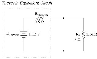
Thevenin's Theorem is especially useful in analyzing power systems and other circuits where one particular resistor in the circuit (called the “load” resistor) is subject to change, and re-calculation of the circuit is necessary with each trial value of load resistance, to determine voltage across it and current through it. Let's take another look at our example circuit:

Thevenin's Theorem makes this easy by temporarily removing the load resistance from the original circuit and reducing what's left to an equivalent circuit composed of a single voltage source and series resistance. The load resistance can then be re-connected to this “Thevenin equivalent circuit” and calculations carried out as if the whole network were nothing but a simple series circuit:


The Thevenin equivalent circuit, if correctly derived, will behave exactly the same as the original circuit formed by B1, R1, R3, and B2. In other words, the load resistor (R2) voltage and current should be exactly the same for the same value of load resistance in the two circuits. The load resistor R2 cannot “tell the difference” between the original network of B1, R1, R3, and B2, and the Thevenin equivalent circuit of EThevenin, and RThevenin, provided that the values for EThevenin and RThevenin have been calculated correctly.
The advantage in performing the “Thevenin conversion” to the simpler circuit, of course, is that it makes load voltage and load current so much easier to solve than in the original network. Calculating the equivalent Thevenin source voltage and series resistance is actually quite easy. First, the chosen load resistor is removed from the original circuit, replaced with a break (open circuit):


Saturday, September 19, 2015
Linearity property
This property gives linear and nonlinear circuit definition. The property can be applied in various circuit elements. The homogeneity (scaling) property and the additive property are both the combination of linearity property.The homogeneity property is that if the input is multiplied by a constant k then the output is also multiplied by the constant k. Input is called excitation and output is called response here. As an example if we consider ohm’s law. Here the law relates the input i to the output v.
ohm's law:
v= iR
If we multiply the input current i by a constant k then the output voltage also increases correspondingly by the constant k. The equation stands,
kiR = kv
The additive property is that the response to a sum of inputs is the sum of the responses to each input applied separately.
Using voltage-current relationship of a resistor if
v1 = i1R and v2 = i2R
Applying (i1 + i2) gives
V = (i1 + i2) R = i1R+ i2R = v1 + v2
Example:

The linear circuit is excited by another outer voltage source vs. Here the voltage source vs acts as input. The circuit ends with a load resistance R. we can take the current I through R as the output.
Suppose vs = 5V and i = 1A. According to linearity property if the voltage is multiplied by 2 then the voltage vs = 10V and then the current also will be multiplied by 2 hence i = 2A.
The power relation is nonlinear. For example, if the current i1 flows through the resistor R, the power p1 = i12R and when current i2 flows through the resistor R then power p2 = i22R.
If the current (i1 + i2) flows through R resistor the power absorbed
P3 = R(i1 + i2)2 = Ri12 + Ri22 + 2Ri1i2 ≠ p1 + p2
So the power relation is nonlinear.
ohm's law:
v= iR
If we multiply the input current i by a constant k then the output voltage also increases correspondingly by the constant k. The equation stands,
kiR = kv
The additive property is that the response to a sum of inputs is the sum of the responses to each input applied separately.
Using voltage-current relationship of a resistor if
v1 = i1R and v2 = i2R
Applying (i1 + i2) gives
V = (i1 + i2) R = i1R+ i2R = v1 + v2
Example:

Suppose vs = 5V and i = 1A. According to linearity property if the voltage is multiplied by 2 then the voltage vs = 10V and then the current also will be multiplied by 2 hence i = 2A.
The power relation is nonlinear. For example, if the current i1 flows through the resistor R, the power p1 = i12R and when current i2 flows through the resistor R then power p2 = i22R.
If the current (i1 + i2) flows through R resistor the power absorbed
P3 = R(i1 + i2)2 = Ri12 + Ri22 + 2Ri1i2 ≠ p1 + p2
So the power relation is nonlinear.
Learnings:
The linear property is similar to an algebraic linear equation. The power of any element shoots up or down in a constant manner thus a circuit has linear property.
Source Transformation
The Source transformation of a circuit is the transformation of a power source from a voltage source to a current source, or a current source to a voltage source.
In other words, we transform the power source from either voltage to current, or current to voltage.
Voltage Source Transformation
We will first go over voltage source transformation, the transformation of a circuit with a voltage source to the equivalent circuit with a current source.
In order to get a visual example of this, let's take the circuit below which has a voltage source as its power source:

Using source transformation, we can change or transform this above circuit with a voltage power source and a resistor, R, in series, into the equivalent circuit with a current source with a resistor, R, in parallel, as shown below:
 We transform a voltage source into a current source by using ohm's law. A voltage source can be changed into a current source by using ohm's formula,I=V/R.
In other words, we transform the power source from either voltage to current, or current to voltage.
Voltage Source Transformation
We will first go over voltage source transformation, the transformation of a circuit with a voltage source to the equivalent circuit with a current source.
In order to get a visual example of this, let's take the circuit below which has a voltage source as its power source:

Learnings:
Source transformation is a good way of solving a circuit as well. However it is not that space friendly because you have to draw a lot of equivalent circuits to simplify extremely your circuit. Also it takes time, but using other solutions still takes up time so if this is easier, we will use it instead.
Superposition
The superposition principle states that the voltage across (or current through) an element in a linear circuit is the algebraic sum of the voltages across (or currents through) that element due to each independent source acting alone.


Learnings:
Superposition is a tricky method because you need to master from basic to nodal or mesh analysis. You need to turn off one power source at a time and sum all the voltages or currents. For us superposition is very useful in my field because superposition is like all the powerplants in the grid when one is turned off what would be the output .Saturday, August 15, 2015
Mesh Analysis
Mesh analysis provides another general procedure for analyzing circuits, using mesh currents as the circuit variables. Using mesh currents instead of element currents as circuit variables is convenient and
reduces the number of equations that must be solved simultaneously. Recall that a loop is a closed path with no node passed more than once. A mesh is a loop that does not contain any other loop within it.


reduces the number of equations that must be solved simultaneously. Recall that a loop is a closed path with no node passed more than once. A mesh is a loop that does not contain any other loop within it.


Learnings:
For us mesh analysis is one of the easiest technique to solve a complicated circuit. We would just loop it, mesh is a loop which doesn't contain another loop inside it anyways, and can solve the circuit with algebra alone. But when asked to find the voltage in a resistor, nodal analysis is our bet.Saturday, July 25, 2015
Nodal Analysis with Voltage source
Greetings our beloved instructor! At last the final topic for the midterm has come. Yet we know it is too early to celebrate because we still have a long way to go. But nevertheless we are quite relieved knowing our coverage for the exams.
Doing nodal analysis can be achieve in two ways, Kirchhoff's current law and Kirchhoff's voltage law. These laws has been discussed on our earlier topics so we assume that elaboration is of no significance anymore. Knowing such we can continue to nodal analysis with voltage source. Of course steps in doing nodal analysis are the following.
vn-1 to the remaining n-1 nodes. The voltages are referenced with respect to the reference node.
2.Apply KCL to each of the n-1 non-reference nodes. Use Ohm’s law to express currents in terms of node voltages.
3. Solve the resulting simultaneous equations to obtain the unknown node voltages.

A Super-node is formed by enclosing a (dependent or independent) voltage source connected between two non-reference nodes and any elements connected in parallel with it.

Step 1. Take off all voltage sources in super-nodes and apply KCL to super-nodes.
Step 2. Put voltage sources back to the nodes and apply KVL to relative loops.

Doing nodal analysis can be achieve in two ways, Kirchhoff's current law and Kirchhoff's voltage law. These laws has been discussed on our earlier topics so we assume that elaboration is of no significance anymore. Knowing such we can continue to nodal analysis with voltage source. Of course steps in doing nodal analysis are the following.
Steps in Nodal Analysis
1. Select a node as the reference node, Assign voltages v1, v2, . . . . . ,vn-1 to the remaining n-1 nodes. The voltages are referenced with respect to the reference node.
2.Apply KCL to each of the n-1 non-reference nodes. Use Ohm’s law to express currents in terms of node voltages.
3. Solve the resulting simultaneous equations to obtain the unknown node voltages.
In nodal analysis with voltage source, we are presented with two cases;
Nodal Analysis with Voltage source Cases:
Case 1:
If the voltage source (dependent or independent) is connected between two non-reference nodes, the two non-reference nodes form a generalized node or super node, we apply both KCL and KVL to determine the node voltages.
Presented in this example.

Case 2:
if a voltage source is connected between the reference node and a non-reference node, we simply set the voltage at the non-reference node equal to the voltage of the voltage sourceA Super-node is formed by enclosing a (dependent or independent) voltage source connected between two non-reference nodes and any elements connected in parallel with it.

Steps in calculating voltage drops on supernodes:
Step 1. Take off all voltage sources in super-nodes and apply KCL to super-nodes.Step 2. Put voltage sources back to the nodes and apply KVL to relative loops.
As shown in this illustration:

Learning:
This week we have learned another nodal analysis but this time with a voltage source. It is quite similar to nodal analysis with current source,but nodal analysis with voltage source will have a supernode, which is a combination of two non-reference nodes connected to the same voltage source. And will have another solution by introducing KVL to the computation together with the KCL on the supernodes. Aside from those, nodal analysis with voltage source is similar to our last week's topic, nodal analysis with current source.
Doing and solving for the values (i.e. voltage drop and current) across a circuit is a lot of fun! We know these topics will help us push through our ever dearly loved careers. Though it is hard at first, we know we can achieve such if we put our utmost effort unto it. It has been said that if there is a will, there is and will always have a way.
Doing and solving for the values (i.e. voltage drop and current) across a circuit is a lot of fun! We know these topics will help us push through our ever dearly loved careers. Though it is hard at first, we know we can achieve such if we put our utmost effort unto it. It has been said that if there is a will, there is and will always have a way.
Saturday, July 18, 2015
Nodal Analysis
Our fine greetings! Today we have again have an amazing week with an also amazing spectacular topic. And it is the nodal analysis, one of the techniques we will have to use in order to calculate the values of any elements we would like in a given more seemingly complicated circuit.
Without further ado, nodal analysis is one of the many methods in solving and finding a specific value of a parameter in electronic circuit analysis. The aim of using nodal analysis is to determine the voltage in each node that’s relative to the reference node, which is the ground GND where voltage is equal to 0. This means that all the other nodes present in the circuit are referred to as the non-reference nodes; the ones that has voltage you are trying to solve for. Depends, of course, if you do need the voltage present in them or not.
Let’s do a quick recap about the parts of an electronic circuit; A node is a point of connection between two or more branches. A branch represents a single element such as a voltage source, or a resistor, etc. And a loop is any closed path in a circuit.
Here are the steps on how to determine node voltages:
Determine the nodes of the circuit, and then select a node as the reference node (ground GND). Then assign the non-reference nodes to voltages V1, V2, Vx, or whatever you feel comfortable with.
Apply KCL (Kirchhoff’s Current Law) to each of the non-reference nodes. Use Ohm’s law (V=IR) to express the branch currents in terms of node voltages. I use the shortcut method, though the same principles are still applied.
Solve the resulting simultaneous equations formed from the non-reference nodes to obtain the unknown node voltages.
Always remember that the number of equations formed should be equal to the number of unknowns. So, taking this simple circuit as an example:

So, there are four nodes. If we were to select the top-left node as the GND, V1 as the top-mid node, V2 as the top-right node, and V3 as the bottom node, it would mean that we can get the voltage across the capacitor with V1 – V3 where V3 = -Vs (voltage source, since the negative terminal of the voltage source is connected to node V3). This would be a fine option but it’s kind of — maybe, unethical — to have the GND connected to the positive terminal of the voltage source.
If we were to select the top-mid node as the GND, V1 as the top-right, and the same position for V2 and V3, then a supernode (formed by enclosing a voltage source, either dependent or independent, connected between two non-reference nodes and any elements connected in parallel with it) would be present which adds more difficulty in solving the circuit. Same situation goes if the top-right node is the GND.
But if we were to select the bottom node as the GND, and V1, V2, and V3 as the top-left, top-mid, and top-right nodes, respectively, then we can get the voltage across the capacitor with V2 – GND = V2 – 0 = V2 (since current flows from a higher potential to a lower potential in a resistor), while V1 = Vs (since the positive terminal of the voltage source is connected to node V1). That makes two unknowns (V2 and V3), though we only need to solve for V2. And it’s more ethical compared to having the GND on top of the circuit.
Now to label the nodes and elements, assuming that all the elements’ respective values are given and have been converted to their equal impedances already. If you want to know how to solve for the impedance in a resistor, inductor, and a capacitor, click here.

@node V2:
V2( ) = 0
To form the equation at node V2, you must locate V2 (imagine V2 as a person or an animal or any object) and look around its surroundings. And I mean the lines or pathways that are connected to it. In this case, there are three pathways connected to V2 (path to V1, to V3, and to GND). And each path is connected to an element (resistor, inductor, and capacitor), or what I will be naming as a bridge. And this is how you start the equation:
V2( 1/bridge1 + 1/bridge2 + 1/bridge3) = 0
..or..
V2( 1/z1 + 1/z2 + 1/z3 ) = 0
It’s like connecting impedances in parallel. Continuing to the path across one of the bridges, you’ll encounter another node (it could either be the GND or not), or what i’ll be naming as your neighbour. This is how neighbours are treated in the equation:
V2( 1/z1 + 1/z2 + 1/z3 ) – neighbour1/bridge1 – neighbour2/bridge2 – neighbour3/bridge3 = 0
..or..
V2( 1/z1 + 1/z2 + 1/z3 ) – V1/z1 – V3/z2 – GND/z3 = 0
..and since V1 = Vs, and GND = 0..
V2( 1/z1 + 1/z2 + 1/z3 ) – Vs/z1 – V3/z2 – 0 = 0
..and since Vs/z1 is a constant, we transpose it to the other side..
V2( 1/z1 + 1/z2 + 1/z3 ) – V3/z2 = Vs/z1
And that’s it for the first equation, with V2 and V3 as unknowns. As I mentioned earlier, the number of unknowns should be equal to the number of equations. So, we are going to need one more equation, and that’d be the equation at node V3.
@node V3:
V3( ) = 0
Following the same procedures with the bridges and neighbours, we get–
V3( 1/z2 ) – V2/z2 = 0
As you can see, node V3 is connected to a current source. A current source in nodal analysis is considered as a constant unless it’s a dependent source. When the current source’s direction is away from the node, you add the current to the equation. If its direction is towards the node, you subtract the current to the equation. And since the current source in the sample circuit is directed towards node V3, it goes like this:
V3( 1/z2 ) – V2/z2 – Is = 0
..and since Is is already a given constant, we transpose it to the other side..
Vs( 1/z2 ) – V2/z2 = Is
And there’s your second equation. Now you can solve for Vz3 by fusing the two equations using matrices, substitution, elimination, or whatever method you know. Though our professor requires us to use the matrix method.
Without further ado, nodal analysis is one of the many methods in solving and finding a specific value of a parameter in electronic circuit analysis. The aim of using nodal analysis is to determine the voltage in each node that’s relative to the reference node, which is the ground GND where voltage is equal to 0. This means that all the other nodes present in the circuit are referred to as the non-reference nodes; the ones that has voltage you are trying to solve for. Depends, of course, if you do need the voltage present in them or not.
Let’s do a quick recap about the parts of an electronic circuit; A node is a point of connection between two or more branches. A branch represents a single element such as a voltage source, or a resistor, etc. And a loop is any closed path in a circuit.
Here are the steps on how to determine node voltages:
Determine the nodes of the circuit, and then select a node as the reference node (ground GND). Then assign the non-reference nodes to voltages V1, V2, Vx, or whatever you feel comfortable with.
Apply KCL (Kirchhoff’s Current Law) to each of the non-reference nodes. Use Ohm’s law (V=IR) to express the branch currents in terms of node voltages. I use the shortcut method, though the same principles are still applied.
Solve the resulting simultaneous equations formed from the non-reference nodes to obtain the unknown node voltages.
Always remember that the number of equations formed should be equal to the number of unknowns. So, taking this simple circuit as an example:

This sample circuit has an AC voltage source, a current source, a resistor, an inductor, and a capacitor. We can also observe that there are four nodes present in this circuit. Assuming that we need to find the voltage across the capacitor, what node will we choose as our reference node GND that will make the problem easier? Note that the lesser the unknowns, the easier the problem will be. It’s like the unknowns determine the difficulty of the problem.
So, there are four nodes. If we were to select the top-left node as the GND, V1 as the top-mid node, V2 as the top-right node, and V3 as the bottom node, it would mean that we can get the voltage across the capacitor with V1 – V3 where V3 = -Vs (voltage source, since the negative terminal of the voltage source is connected to node V3). This would be a fine option but it’s kind of — maybe, unethical — to have the GND connected to the positive terminal of the voltage source.
If we were to select the top-mid node as the GND, V1 as the top-right, and the same position for V2 and V3, then a supernode (formed by enclosing a voltage source, either dependent or independent, connected between two non-reference nodes and any elements connected in parallel with it) would be present which adds more difficulty in solving the circuit. Same situation goes if the top-right node is the GND.
But if we were to select the bottom node as the GND, and V1, V2, and V3 as the top-left, top-mid, and top-right nodes, respectively, then we can get the voltage across the capacitor with V2 – GND = V2 – 0 = V2 (since current flows from a higher potential to a lower potential in a resistor), while V1 = Vs (since the positive terminal of the voltage source is connected to node V1). That makes two unknowns (V2 and V3), though we only need to solve for V2. And it’s more ethical compared to having the GND on top of the circuit.
Now to label the nodes and elements, assuming that all the elements’ respective values are given and have been converted to their equal impedances already. If you want to know how to solve for the impedance in a resistor, inductor, and a capacitor, click here.

There we go! So, what we are trying to find is the voltage across the capacitor Z3 and we have discussed earlier that Vz3 = V2, since Vz3 = V2 – GND and that the voltage at the GND is equal to 0. Now to form the equation at node V2 using the shortcut method. Brace yourself for I am about to make up names that i’ll be using to better explain the shortcut method.
@node V2:
V2( ) = 0
To form the equation at node V2, you must locate V2 (imagine V2 as a person or an animal or any object) and look around its surroundings. And I mean the lines or pathways that are connected to it. In this case, there are three pathways connected to V2 (path to V1, to V3, and to GND). And each path is connected to an element (resistor, inductor, and capacitor), or what I will be naming as a bridge. And this is how you start the equation:
V2( 1/bridge1 + 1/bridge2 + 1/bridge3) = 0
..or..
V2( 1/z1 + 1/z2 + 1/z3 ) = 0
It’s like connecting impedances in parallel. Continuing to the path across one of the bridges, you’ll encounter another node (it could either be the GND or not), or what i’ll be naming as your neighbour. This is how neighbours are treated in the equation:
V2( 1/z1 + 1/z2 + 1/z3 ) – neighbour1/bridge1 – neighbour2/bridge2 – neighbour3/bridge3 = 0
..or..
V2( 1/z1 + 1/z2 + 1/z3 ) – V1/z1 – V3/z2 – GND/z3 = 0
..and since V1 = Vs, and GND = 0..
V2( 1/z1 + 1/z2 + 1/z3 ) – Vs/z1 – V3/z2 – 0 = 0
..and since Vs/z1 is a constant, we transpose it to the other side..
V2( 1/z1 + 1/z2 + 1/z3 ) – V3/z2 = Vs/z1
And that’s it for the first equation, with V2 and V3 as unknowns. As I mentioned earlier, the number of unknowns should be equal to the number of equations. So, we are going to need one more equation, and that’d be the equation at node V3.
@node V3:
V3( ) = 0
Following the same procedures with the bridges and neighbours, we get–
V3( 1/z2 ) – V2/z2 = 0
As you can see, node V3 is connected to a current source. A current source in nodal analysis is considered as a constant unless it’s a dependent source. When the current source’s direction is away from the node, you add the current to the equation. If its direction is towards the node, you subtract the current to the equation. And since the current source in the sample circuit is directed towards node V3, it goes like this:
V3( 1/z2 ) – V2/z2 – Is = 0
..and since Is is already a given constant, we transpose it to the other side..
Vs( 1/z2 ) – V2/z2 = Is
And there’s your second equation. Now you can solve for Vz3 by fusing the two equations using matrices, substitution, elimination, or whatever method you know. Though our professor requires us to use the matrix method.
Learning:
This week we have learned to use another method, called nodal analysis in solving some values of the elements present in the circuit. The first process we need to do is to locate a reference node, a node where most of the elements are connected, second is to assign voltages across each non-reference nodes. Third is to use KCL on each non-reference nodes. Lastly in order to solve for the voltages on each nodes, we are required to use the matrix and do the math. :D
Friday, July 10, 2015
Basic Laws: Wye-Delta Transformation II
CET acquaintance is coming! So we decided to make this blog a day earlier because we might be too tired to do stuffs after the event. Anyways. Greetings again our dear professor! We got a problem upon discussing what to write on this blog for because the topic that we discussed last week, is of the same topic we have discussed this week. But as we specified on our last blog, the wye-delta transformation that we have explained is only a kind of introduction. So now we decided to make wye-delta transformation a little broader.


PROPER USAGE OF WYE-DELTA TRANSFORMATION
How to apply this wye-delta transformation? Lets have this example.

As said, we use wye-delta transformation if the resistors are neither connected in series or parallel. Thus getting the equivalent resistance may seem impossible if wye-delta transformation is not applied. On the given example, we first determine what is the best and easiest transformation in order to acquire the equivalent resistance. On this case, delta to wye transformation is the likely candidate, because in only one transformation we can solve directly the equivalent resistance. Also there are no wye (Y) circuit formation found on the circuit. Never realized that one until few seconds ago. Anyways applying these equation to R1, R2 and R3 we can arrive at a redrawn but equivalent circuit.
Thus the redrawn circuit will look like.

Our deepest apologies for a badly made redrawn circuit. Now we can actually solve for the equivalent resistance which is simply.
However, this equation is only applicable to our redrawn circuit.
Learning:
This week (although we had similar topic of the previous week) we have learned that doing wye-delta is not complicated as it first seems. The only weight is to analyze the circuit and understand what transformation should be used for us to acquire and be able to have the equivalent resistance of the circuit.
"Having to deal with technology can be painfully harsh, but every pain has its own hidden worth"
Saturday, July 4, 2015
Basic Law: Wye-Delta Transformation
Good evening! Or good noon? morning? We don’t even know anymore. Should we greet with the time setting of when we made this blog, or when will you sir, our professor, will be reading our blogs? But of course we would not know when will you read so to be safe we would just rather say.
Greetings our beloved instructor! A week has passed again, and we are now on a new topic. Well it was kind of an introduction, we presume. Because Wednesday this week we had our first ever quiz, which by the way, we failed so hard. But maybe that is a challenge for us, to work harder, to be better! Or we did just failed the first quiz miserably. Anyways, our new topic is about:
Situations often arise in circuit analysis when the resistors are neither in parallel nor in series. This situations are where this wye-delta transformation technique is used, where it simplifies the analysis of an electric network or circuit. The Y-Δ transformation is known by a variety of other names, mostly based upon the two shapes involved, listed in either order. The Y, spelled out as wye, can also be called T or star; the Δ, spelled out as delta, can also be called triangle, Π (spelled out as pi), or mesh. Thus, common names for the transformation include wye-delta or delta-wye, star-delta, star-mesh, or T-Π. The concept is to transform a wye (y) electric network into a delta (Δ) electric network and vice versa in order to evaluate the circuit.


Greetings our beloved instructor! A week has passed again, and we are now on a new topic. Well it was kind of an introduction, we presume. Because Wednesday this week we had our first ever quiz, which by the way, we failed so hard. But maybe that is a challenge for us, to work harder, to be better! Or we did just failed the first quiz miserably. Anyways, our new topic is about:
WYE-DELTA TRANSFORMATION
Situations often arise in circuit analysis when the resistors are neither in parallel nor in series. This situations are where this wye-delta transformation technique is used, where it simplifies the analysis of an electric network or circuit. The Y-Δ transformation is known by a variety of other names, mostly based upon the two shapes involved, listed in either order. The Y, spelled out as wye, can also be called T or star; the Δ, spelled out as delta, can also be called triangle, Π (spelled out as pi), or mesh. Thus, common names for the transformation include wye-delta or delta-wye, star-delta, star-mesh, or T-Π. The concept is to transform a wye (y) electric network into a delta (Δ) electric network and vice versa in order to evaluate the circuit.

Basic Y-Δ transformation

The transformation is used to establish equivalence for networks with three terminals. Where three elements terminate at a common node and none are sources, the node is eliminated by transforming the impedances. For equivalence, the impedance between any pair of terminals must be the same for both networks. The equations given here are valid for complex as well as real impedances. Impedance actually is the measure of the opposition that a circuit presents to a current when a voltage is applied. In quantitative terms, it is the complex ratio of the voltage to the current in an alternating current (AC) circuit.
But in order to transform wye-delta or delta-wye. We must use a solution, transforming each would require that even if it is transformed, the elements would still be of equal value.
Equations for the transformation from Δ to Y
Equations for the transformation from Y to Δ
Learning:
This week we are introduced to a new way of reconstructing a circuit. It is called the wye-delta transformation. This transformation is used in order to reconstruct the resistance on the circuit to be able to calculate the equivalent resistance present on a seemingly complicated circuit. However just barely transforming wye-delta or delta-wye configurations of any given resistors may give or may not give you the desired configuration of the circuit to be able to calculate the equivalent resistance. A better understanding of how the resistors are connected and analyzing which way are the best is crucial in complicated circuits.
We are new to circuits and we still have a lot to learn. But with every new method, we are bound to unlock more understanding of what and how can we do better in this program.
“We are doing our best! So please grades, do catch up” – every engineering student ever.
Saturday, June 27, 2015
Basic Law (Series and Parallel Resistors)
It’s been another week! And here we are again with our weekly dose in everything about circuits. Every little thing is so important that we have to master every bit of it. Specially on the prelude part, or the introduction parts, the basics is at most priority. The basic laws, as our beloved professor would say, without mastering these basic laws, we will have difficulties on the future matters.
The first law that we learned is the series resistor connection or simply put series connection. A connection is said to be series if the current is flowing on a single path and has the same amount through the connection. And we also learned that (although it was then thought on our physics class, but it is good that we have some refreshment of such) in a series connection, it will have the same current flowing on it, but it will have different voltages across each resistors. Thus we learned about voltage division. Voltage division is the formula (at least that is what we know of it) that can accurately solve for each of such voltage across resistors. It is written in V1=VR1(R1+R2), where “R” is a the amount of resistance a resistor and “V” obviously is a voltage. To solve for equivalent resistance (Req) for a series connection, here is the formula, Req=R1+R2 … . And often we only use the ohm’s law to solve for voltage, resistance and current.
Series connection is as illustrated as follows.

The second law that we learned is the parallel resistor connection or simply put parallel connection. A connection is said to be parallel if the voltage flowing is common across the connection. Also the current flows in two or more path along the connection. As said, the voltage across each resistors are the same, but the current flowing on each will have different values thus we have been introduced to the current division. Current division is a formula (or at least that is what we know of it) that can accurately solve for each of such current across resistors. It is written in I1=IR2/(R1+R2), where ”R” is a the amount of resistance a resistor and I is obviously the current. To solve for its equivalent resistance (Req) of a parallel connection the formula to be used is, 1/Req=1/R1+1/R2 … . And the used formula to solve for any voltage, current, resistance is the Kirchhoff’s Voltage Law(KVL) and Kirchhoff’s Current Law(KCL).
Parallel connection is as illustrated as follows.

The first law that we learned is the series resistor connection or simply put series connection. A connection is said to be series if the current is flowing on a single path and has the same amount through the connection. And we also learned that (although it was then thought on our physics class, but it is good that we have some refreshment of such) in a series connection, it will have the same current flowing on it, but it will have different voltages across each resistors. Thus we learned about voltage division. Voltage division is the formula (at least that is what we know of it) that can accurately solve for each of such voltage across resistors. It is written in V1=VR1(R1+R2), where “R” is a the amount of resistance a resistor and “V” obviously is a voltage. To solve for equivalent resistance (Req) for a series connection, here is the formula, Req=R1+R2 … . And often we only use the ohm’s law to solve for voltage, resistance and current.
Series connection is as illustrated as follows.

The second law that we learned is the parallel resistor connection or simply put parallel connection. A connection is said to be parallel if the voltage flowing is common across the connection. Also the current flows in two or more path along the connection. As said, the voltage across each resistors are the same, but the current flowing on each will have different values thus we have been introduced to the current division. Current division is a formula (or at least that is what we know of it) that can accurately solve for each of such current across resistors. It is written in I1=IR2/(R1+R2), where ”R” is a the amount of resistance a resistor and I is obviously the current. To solve for its equivalent resistance (Req) of a parallel connection the formula to be used is, 1/Req=1/R1+1/R2 … . And the used formula to solve for any voltage, current, resistance is the Kirchhoff’s Voltage Law(KVL) and Kirchhoff’s Current Law(KCL).
Parallel connection is as illustrated as follows.

Learning:
Another basic we have to master. Knowing the current flow to each elements is the key in knowing if a connection is parallel in each other or in series with themselves. The current that flows (picture out a current as a flow of water) in a series connection, same current flows on each elements. Similar to a water that flows on a single path. In a parallel connection, different current flows on each element. Similar to a water flow that splits in two or more direction, the water flow will differ from stream to streams with respect to the area, altitude and any other aspects that minimizes the flow of the water, it is also holds true on a parallel connection but is called resistance.
“If we love our job and what we do. We will never have to work anymore.”-AnonymousFriday, June 19, 2015
Prelude to Circuits 1 (Ohm's Law, KVL/KCL)
Welcome sir to our first and not so good blog.
We’ve just been studying electrical circuits for about one week, but we have learned so much in just this few days.
Let us start with the meaning of “Electrical Circuit” and its basic units that will be used mostly throughout this semester, if what we believed is true.
For the head start, “Electric circuit” is the interconnection of “circuit elements” which is the basic building blocks of a circuit. This includes the resistors, power source, the electrical/connecting wires and many more and is divided into three types, the “active” which is capable of generating energy, “passive” which absorbs energy, and the “V and I sources” that is the most important active element.
For its basic units, first we have the “Charge”, on other language charge is something used as alternative for paying. Like we are charged 1000 php for purchasing a video game. But in electrical circuits, charge is used differently. Charge in such is defined as the basic quantity of an electric circuits. This means that whatever we measure in our electric circuit, there will always be the presence of charge. And we realized that this “charge” is at most important especially for the likes of us.
Second is the “Current”, current is “charge” flow rate, and is measured in amperes. We have learned that current is what makes the computer that I am using now work, of course with the help of “Voltage”, the charge rate of doing work and is the third basic unit of circuits that we learned. Also there is this “Power” that is defined by the time rate of doing work along with the “Energy” that is the capacity to do work.
“Sources”, we also have discussed the two types of power sources, the “Independent source” which obviously is independent on other elements to perform and supply power. “Dependent source” that depends on other elements to supply its glorious power.
We also have noticed, that this subject, electrical circuits 1, is connected still to our previous subject specifically the differential and integral calculus and geometries. To be able to make and create our own formula to calculate precisely the behavior of a certain charge or unit.
From that we had to jump to the second chapter of electrical circuits, which covers the basic laws used in electric boards and circuits. These two laws was introduced in one of our subject before, we’ve never been so glad to see such familiar words and equations.
Without such further delay, the first law of circuits is the “Ohms law” which states that the “voltage” is directly proportional to the “current” where “resistance” is the constant of proportionality. In short V=IR, but this law can only be use in linear resistors.
Before we continue to the second law, we first discussed about how the elements of circuits can be interconnected. We have been introduced to three new terms which are the “Branch”, which represents a single element, “Node”, the meeting point between two or more branches, and “Loop”, which is any closed path in a circuit.
And so, the second basic law is the “Kirchhoff’s Law”, which is also divided into two parts, the “Kirchhoff’s Current Law” which is the algebraic sum of all entering/leaving current through a node and the “Kirchhoff’s Voltage Law” which states that in any closed loop network, the total voltage around the loop is equal to the sum of all the voltage drops within the same loop.

We’ve just been studying electrical circuits for about one week, but we have learned so much in just this few days.
Let us start with the meaning of “Electrical Circuit” and its basic units that will be used mostly throughout this semester, if what we believed is true.
For the head start, “Electric circuit” is the interconnection of “circuit elements” which is the basic building blocks of a circuit. This includes the resistors, power source, the electrical/connecting wires and many more and is divided into three types, the “active” which is capable of generating energy, “passive” which absorbs energy, and the “V and I sources” that is the most important active element.
For its basic units, first we have the “Charge”, on other language charge is something used as alternative for paying. Like we are charged 1000 php for purchasing a video game. But in electrical circuits, charge is used differently. Charge in such is defined as the basic quantity of an electric circuits. This means that whatever we measure in our electric circuit, there will always be the presence of charge. And we realized that this “charge” is at most important especially for the likes of us.
Second is the “Current”, current is “charge” flow rate, and is measured in amperes. We have learned that current is what makes the computer that I am using now work, of course with the help of “Voltage”, the charge rate of doing work and is the third basic unit of circuits that we learned. Also there is this “Power” that is defined by the time rate of doing work along with the “Energy” that is the capacity to do work.
“Sources”, we also have discussed the two types of power sources, the “Independent source” which obviously is independent on other elements to perform and supply power. “Dependent source” that depends on other elements to supply its glorious power.
We also have noticed, that this subject, electrical circuits 1, is connected still to our previous subject specifically the differential and integral calculus and geometries. To be able to make and create our own formula to calculate precisely the behavior of a certain charge or unit.
From that we had to jump to the second chapter of electrical circuits, which covers the basic laws used in electric boards and circuits. These two laws was introduced in one of our subject before, we’ve never been so glad to see such familiar words and equations.
Without such further delay, the first law of circuits is the “Ohms law” which states that the “voltage” is directly proportional to the “current” where “resistance” is the constant of proportionality. In short V=IR, but this law can only be use in linear resistors.
Before we continue to the second law, we first discussed about how the elements of circuits can be interconnected. We have been introduced to three new terms which are the “Branch”, which represents a single element, “Node”, the meeting point between two or more branches, and “Loop”, which is any closed path in a circuit.
And so, the second basic law is the “Kirchhoff’s Law”, which is also divided into two parts, the “Kirchhoff’s Current Law” which is the algebraic sum of all entering/leaving current through a node and the “Kirchhoff’s Voltage Law” which states that in any closed loop network, the total voltage around the loop is equal to the sum of all the voltage drops within the same loop.
Learning:
Learning the basics of everything is the key to a brighter future. One will never be able to do algebra, geometry and even calculus without knowing simply how to add, subtract, divide and multiply. In a similar fashion, we will never be able to move forward without know the basics of circuits.
Ohm's Law, which is the most basic formula that we will have to use mostly in this program, states that voltage is directly proportional to the current of course with the resistance as its constant of proportionality. This means that if the voltage increases, the current will also increase in a similar way.
Second is the Kirchhoff's voltage and current law, Kirchhoff's voltage law states that in a close loop or path, the summation of all the voltages is and must be equal to zero. And Kirchhoff's current law states that in a node, the summation of all the current entering such node, is equal to the summation of all the current leaving the node.
Upon knowing the laws, we had a board work that teaches us how to properly use this laws and we learned how important it is specially for us. Gawd! Being an Electronics and Communication Engineering student is hard.Second is the Kirchhoff's voltage and current law, Kirchhoff's voltage law states that in a close loop or path, the summation of all the voltages is and must be equal to zero. And Kirchhoff's current law states that in a node, the summation of all the current entering such node, is equal to the summation of all the current leaving the node.

Subscribe to:
Posts (Atom)